**
**
OS version: Windows 11 - 24H2 - Build 26100.3775 - Expérience Windows 1000.26100.66.0
App version: Desktop version 8.3.3.21 (x64 exe)
Downloaded from: ONLYOFFICE website
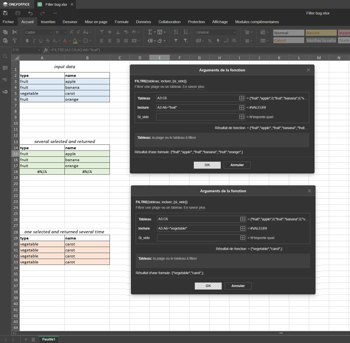
I use function “Filter” on spreadsheet and put the result in an array, the same size of the original array.
When the result of the function return several rows, the resulting array is correct
- green array on the uploaded image, and the parameters of the funcion in the dialog box on the right
When the result of the function is only one element, the resulting array get that element in all rows
- red array on the uploaded image, and the parameters of the funcion in the dialog box on the right
Only one element should be returned in the resulting array, as state in “result of the formula” in the dialog box.
Hello @FrankyCHAMBERS
Would you mind sharing all steps to reproduce the issue? I was not able to reproduce it by simply choosing a single cell and then applying the formula.
To reproduce follow the steps below
- assuming you have the input data array ready
- select range A30:B33
- in the formula bar enter =FILTRE(A3:B6;A3:A6=“vegetable”)
- type CTRL+SHIFT+ENTER to enter the formula as an array formula ={FILTRE(A3:B6;A3:A6=“vegetable”)}
If you don’t select cells range, prior to enter the formula, weird thing happen.
If you put the formula in A30, without selecting range A30:A33 before, the first formula give you 3 rows, it’s correct (and without #N/A in the fourth row)
If you change A30 to the second formula, you get 3 rows populated with the same value.
Inversly, if you enter the second formula first, you get one row, it’s correct. If you then enter the first formula in A30, you get only the first row instead of 3 rows.
It’s as thought the sheet memorises the first number of values returned and uses it for all following computations.
Maybe I am misunderstanding some key aspects, but using any formula (with “fruit” or “vegetable”) and in any order (“fruit” first or vice versa) results in creation of array formula with correct results. Can you record a video demonstration for better understanding of performed steps?
That is strange, I cannot reproduce this behavior. Where did you download the app?
Regular update from https://www.onlyoffice.com/
To reproduce you have to validate the formula by CTRL+SHITF+ENTER i.e validate the formula as an array formula.
Okay, that way it reproduces. However, I am certain that this forceful formatting of the formula into array formula, a.k.a. CSE, is not needed, because regular usage of dynamic formula arrays instead does the job as you’d expect it. CSE remains funcional for compatibility reasons.
As far as I know, this is expected behavior for CSE formulas.
Unfortunately, the result depends of the CSE and array cells selected first.
I need ALL cells populated in the resulting array. The recording show all the senarios.
In my spreadsheet, I bypass this bug by creating another column, with duplicates removed.
I’m afraid this is expected behavior with dynamic arrays formulas compared to CSE. I am referring to appearance of N/A values in cells.
However, I’ve noticed that defining a formula as dynamic array and changing value in the list does not display changes to that array, i.e. when running =FILTER(A1:B4;A1:A4=D4) as “fruit”, it changes values to “fruit” in all three rows, instead of dynamically reducing the array to only 1 row according to the actual result and vice versa. We will check out this behavior.